7 · Gradient descent on a manifold with non-Euclidean geometry#

Tutorial 3 hinted that the gradient depends on the inner product. Here we take that idea all the way: we optimise over a curved manifold equipped with a non-Euclidean metric, and the right search direction is the Riemannian (natural) gradient — the coordinate gradient with its index raised by the inverse metric. In SpaceCore that index-raising is exactly space.riesz_inverse, and the metric is supplied by a custom ``InnerProduct``.

Our manifold is the unit sphere of a metric $M$,

\[\mathcal{S}_M = \{\, x \in \mathbb{R}^3 : \langle x, x\rangle_M = x^\top M x = 1 \,\},\]

(an ellipsoid in ordinary coordinates) and we minimise the linear objective $f(x) = -\,t^\top x$ over it.

You will learn to write a custom geometry, build the Riemannian gradient with riesz_inverse, and run constrained descent with a projection + retraction.

import numpy as np
import matplotlib as mpl
import matplotlib.pyplot as plt
import spacecore as sc

# A clean, consistent palette + style for every figure in the tutorials.
BLUE, INDIGO, CYAN = "#2563eb", "#4f46e5", "#0891b2"
PINK, AMBER, GREEN = "#db2777", "#d97706", "#059669"
SLATE, GRID = "#334155", "#e5e9f0"

mpl.rcParams.update({
    "figure.figsize": (7.2, 4.2), "figure.dpi": 120, "savefig.dpi": 120,
    "figure.facecolor": "white", "axes.facecolor": "white",
    "axes.edgecolor": SLATE, "axes.linewidth": 1.0,
    "axes.grid": True, "axes.axisbelow": True,
    "grid.color": GRID, "grid.linewidth": 1.0,
    "axes.spines.top": False, "axes.spines.right": False,
    "axes.titlesize": 13, "axes.titleweight": "bold", "axes.titlecolor": SLATE,
    "axes.labelcolor": SLATE, "axes.labelsize": 11,
    "xtick.color": SLATE, "ytick.color": SLATE,
    "xtick.labelsize": 10, "ytick.labelsize": 10, "font.size": 11,
    "legend.frameon": False, "legend.fontsize": 10,
    "lines.linewidth": 2.4, "lines.markersize": 6, "image.cmap": "magma",
})
mpl.rcParams["axes.prop_cycle"] = mpl.cycler(
    color=[BLUE, PINK, GREEN, AMBER, INDIGO, CYAN])

print("spacecore", sc.__version__, "| numpy", np.__version__)

spacecore 0.4.0 | numpy 2.4.2

ctx = sc.Context(sc.NumpyOps(), dtype=np.float64)
ops = ctx.ops

1 · A custom metric is a custom `InnerProduct`#

A geometry implements inner (and, to be useful for gradients, riesz / riesz_inverse — the maps that lower and raise indices). Here is a constant SPD metric $\langle x,y\rangle = x^\top M y$; its riesz_inverse is multiplication by $M^{-1}$, which is what turns a coordinate gradient into the natural gradient.

from spacecore.space import InnerProduct

class MatrixInnerProduct(InnerProduct):
    """Constant SPD metric  <x, y> = xᵀ M y."""
    def __init__(self, M):
        self.M = np.asarray(M, dtype=float)
        self.Minv = np.linalg.inv(self.M)
    def inner(self, ops, x, y):       return ops.vdot(x, ops.matmul(ctx.asarray(self.M), y))
    def riesz(self, ops, x):          return ops.matmul(ctx.asarray(self.M), x)     # lower index
    def riesz_inverse(self, ops, x):  return ops.matmul(ctx.asarray(self.Minv), x)  # raise → nat. grad
    def validate_for(self, space):                                                   # light sanity check
        n = int(np.prod(space.shape))
        if self.M.shape != (n, n):
            raise ValueError(f"metric must be {n}x{n}, got {self.M.shape}")
    def convert(self, ctx):           return self
    @property
    def is_euclidean(self):           return False

M = np.array([[2.0, 0.6, 0.0],
              [0.6, 1.0, 0.0],
              [0.0, 0.0, 1.3]])
Sm = sc.DenseVectorSpace((3,), ctx, geometry=MatrixInnerProduct(M))

x = ctx.asarray([1.0, 0.0, 1.0]); y = ctx.asarray([0.0, 1.0, 1.0])
print("<x, y>_M           :", float(Sm.inner(x, y)), " (= xᵀ M y)")
print("riesz_inverse∘riesz:", Sm.riesz_inverse(Sm.riesz(x)), " (round-trips to x)")
print("is_euclidean       :", Sm.is_euclidean)

<x, y>_M           : 1.9  (= xᵀ M y)
riesz_inverse∘riesz: [1. 0. 1.]  (round-trips to x)
is_euclidean       : False

2 · Riemannian gradient descent#

One step on the $M$-sphere has three parts:

raise the index — natural gradient $:raw-latex:nabla_M f = M^{-1}:raw-latex:partial `f = $ ``Sm.riesz_inverse(∂f)`;
project onto the tangent space $\{v : \langle x, v\rangle_M = 0\}$, using the $M$-inner product;
retract back onto the manifold by $M$-normalising.

We run it twice: once with the natural gradient (riesz_inverse), and once with the raw coordinate gradient (the common bug of forgetting to raise the index, which is just Euclidean steepest descent). Both descend, but on different paths.

t = ctx.asarray([0.6, 0.9, 0.4])          # objective f(x) = -tᵀx
f          = lambda x: -float(ops.vdot(t, x))
coord_grad = lambda x: -t                  # ∂f/∂x  (a covector)
m_normalize = lambda x: x / float(np.sqrt(Sm.inner(x, x)))

def riemannian_descent(use_natural, eta=0.35, n_steps=40):
    x = m_normalize(ctx.asarray([0.2, -0.9, 0.3]))
    xs, fs = [np.asarray(x).copy()], [f(x)]
    for _ in range(n_steps):
        g = Sm.riesz_inverse(coord_grad(x)) if use_natural else coord_grad(x)
        coef = Sm.inner(x, g) / Sm.inner(x, x)        # tangent projection (M-orthogonal)
        tan = g - coef * x
        x = m_normalize(x - eta * tan)                # gradient step + retraction
        xs.append(np.asarray(x).copy()); fs.append(f(x))
    return np.array(xs), np.array(fs)

path_nat, f_nat = riemannian_descent(use_natural=True)
path_euc, f_euc = riemannian_descent(use_natural=False)

# closed-form optimum of  max tᵀx  s.t.  xᵀMx = 1
x_star = np.linalg.solve(M, np.asarray(t)); x_star /= np.sqrt(x_star @ M @ x_star)
print("natural-grad final f :", f_nat[-1])
print("Euclidean-grad final f:", f_euc[-1])
print("optimal f*           :", -float(np.asarray(t) @ x_star))
print("on manifold? xᵀMx =", float(path_nat[-1] @ M @ path_nat[-1]))

natural-grad final f : -0.9670946411949166
Euclidean-grad final f: -0.861026308213982
optimal f*           : -0.9670946411950294
on manifold? xᵀMx = 1.0

3 · See it on the manifold#

The $M$-unit sphere is an ellipsoid. We draw it, then trace both descent paths from the same start to the same optimum (green star). The natural-gradient route (pink) honours the metric and takes a more direct path than the metric-blind Euclidean route (blue).

# ellipsoid surface: x = M^{-1/2} y for y on the Euclidean unit sphere
evals, evecs = np.linalg.eigh(M)
M_half_inv = evecs @ np.diag(evals ** -0.5) @ evecs.T
uu, vv = np.mgrid[0:np.pi:40j, 0:2*np.pi:40j]
sph = np.stack([np.sin(uu)*np.cos(vv), np.sin(uu)*np.sin(vv), np.cos(uu)])
ell = np.einsum("ij,jkl->ikl", M_half_inv, sph)

fig = plt.figure(figsize=(11, 4.6))
ax = fig.add_subplot(1, 2, 1, projection="3d")
ax.plot_surface(ell[0], ell[1], ell[2], color=CYAN, alpha=0.12,
                linewidth=0, antialiased=True)
ax.plot_wireframe(ell[0], ell[1], ell[2], color=CYAN, alpha=0.18, linewidth=0.4)
for path, color, lab in [(path_euc, BLUE, "Euclidean gradient"),
                         (path_nat, PINK, "natural gradient")]:
    ax.plot(path[:, 0], path[:, 1], path[:, 2], color=color, lw=2.6, label=lab)
    ax.scatter(*path[0], color=color, s=30)
ax.scatter(*x_star, color=GREEN, s=140, marker="*", label="optimum")
ax.set_title("Descent on the $M$-unit sphere"); ax.legend(loc="upper left", fontsize=8)
ax.set_xticks([]); ax.set_yticks([]); ax.set_zticks([])

ax2 = fig.add_subplot(1, 2, 2)
opt = -float(np.asarray(t) @ x_star)
ax2.semilogy(f_euc - opt + 1e-16, color=BLUE, marker="o", ms=3, label="Euclidean gradient")
ax2.semilogy(f_nat - opt + 1e-16, color=PINK, marker="o", ms=3, label="natural gradient")
ax2.set_title("Suboptimality  $f(x_k) - f^\\star$"); ax2.set_xlabel("iteration")
ax2.set_ylabel("gap (log)"); ax2.legend()
plt.tight_layout(); plt.show()

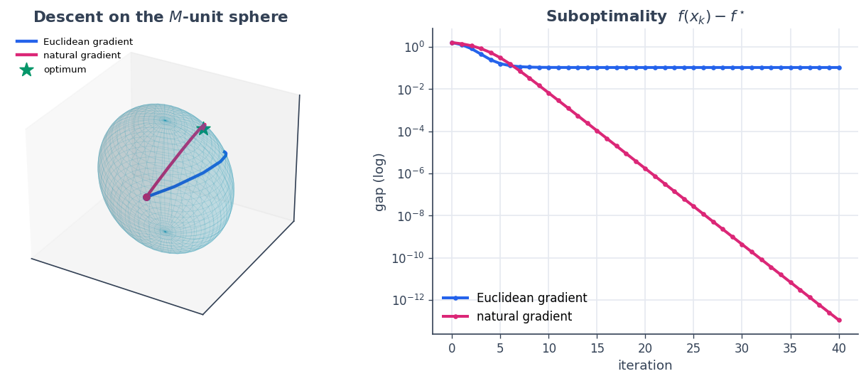
Both paths stay exactly on the ellipsoid (we checked $x^\top M x = 1$) and reach the same optimum, but the natural gradient — built with a single call to riesz_inverse — gets there in fewer, straighter steps. The metric is not a detail; it is the descent direction.

State-dependent metrics. A Space’s geometry is fixed, so it models a constant metric. For a metric that varies with position (e.g. Fisher–Rao on the probability simplex, where $G(p)=\mathrm{diag}(1/p)$), rebuild a WeightedInnerProduct space at each iterate — the natural gradient is still just riesz_inverse of the coordinate gradient.

Recap#

A non-Euclidean geometry is a custom ``InnerProduct``: implement inner, riesz, riesz_inverse, is_euclidean, and validate_for.
The natural / Riemannian gradient is space.riesz_inverse(coordinate_gradient) — raising the index with the inverse metric.
Manifold descent = natural gradient → tangent projection → retraction; the metric shapes both the manifold and the path.

Next: 8 · PDHG for a conic program — operators, cones, and a primal–dual saddle point.

7 · Gradient descent on a manifold with non-Euclidean geometry#

1 · A custom metric is a custom InnerProduct#

2 · Riemannian gradient descent#

3 · See it on the manifold#

Recap#

1 · A custom metric is a custom `InnerProduct`#