4 · Tree spaces: structured elements and block operators#
Not every unknown is a flat vector. A saddle-point system has a primal
block and a dual block of different sizes; a PDE solve might carry a
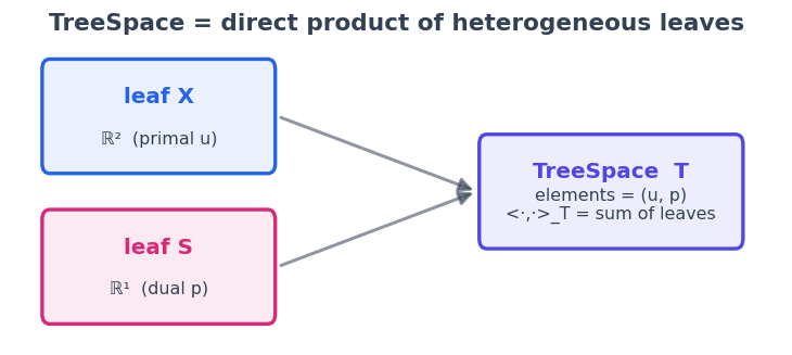
field plus a handful of scalar multipliers. A ``TreeSpace`` is the
direct product of heterogeneous leaf spaces, organised as a Python tree
(a tuple, list, dict, or NamedTuple). Its elements are trees of
arrays; its inner product is the sum of the leaf inner products; and
block operators map one tree space to another.
We will assemble a \(2\times 2\) block SPD system
with \(u \in \mathbb{R}^2\) and \(p \in \mathbb{R}^1\) living in
different leaves, and solve it with sc.cg directly over the tree
space.
You will learn to build a TreeSpace and TreeElement, compose
blocks with BlockMatrixLinOp, and run a Krylov solver over
structured unknowns.
import numpy as np
import matplotlib as mpl
import matplotlib.pyplot as plt
import spacecore as sc

# A clean, consistent palette + style for every figure in the tutorials.
BLUE, INDIGO, CYAN = "#2563eb", "#4f46e5", "#0891b2"
PINK, AMBER, GREEN = "#db2777", "#d97706", "#059669"
SLATE, GRID = "#334155", "#e5e9f0"

mpl.rcParams.update({
    "figure.figsize": (7.2, 4.2), "figure.dpi": 120, "savefig.dpi": 120,
    "figure.facecolor": "white", "axes.facecolor": "white",
    "axes.edgecolor": SLATE, "axes.linewidth": 1.0,
    "axes.grid": True, "axes.axisbelow": True,
    "grid.color": GRID, "grid.linewidth": 1.0,
    "axes.spines.top": False, "axes.spines.right": False,
    "axes.titlesize": 13, "axes.titleweight": "bold", "axes.titlecolor": SLATE,
    "axes.labelcolor": SLATE, "axes.labelsize": 11,
    "xtick.color": SLATE, "ytick.color": SLATE,
    "xtick.labelsize": 10, "ytick.labelsize": 10, "font.size": 11,
    "legend.frameon": False, "legend.fontsize": 10,
    "lines.linewidth": 2.4, "lines.markersize": 6, "image.cmap": "magma",
})
mpl.rcParams["axes.prop_cycle"] = mpl.cycler(
    color=[BLUE, PINK, GREEN, AMBER, INDIGO, CYAN])

print("spacecore", sc.__version__, "| numpy", np.__version__)
spacecore 0.4.0 | numpy 2.4.2
ctx = sc.Context(sc.NumpyOps(), dtype=np.float64)
1 · A space made of spaces#
TreeSpace.from_leaf_spaces((X, S)) glues leaf spaces into a
tuple-structured product. An element is just a tuple (u, p) of leaf
arrays.
X = sc.DenseVectorSpace((2,), ctx)        # primal leaf  u ∈ ℝ²
S = sc.DenseVectorSpace((1,), ctx)        # dual leaf    p ∈ ℝ¹
T = sc.TreeSpace.from_leaf_spaces((X, S), ctx)

u = (ctx.asarray([1.0, 2.0]), ctx.asarray([3.0]))
v = (ctx.asarray([4.0, 5.0]), ctx.asarray([6.0]))

print("leaf paths :", T.leaf_paths)
print("<u, v>_T   :", T.inner(u, v), " (= 1·4 + 2·5 + 3·6 — sum over leaves)")
print("||u||_T    :", T.norm(u))
print("flatten    :", T.flatten(u), " (tree → one dense vector)")
print("zeros      :", T.zeros())

el = sc.TreeElement(T, u)                 # an explicit element bound to its space
print("element    :", el.value)
leaf paths : ((0,), (1,))
<u, v>_T   : 32.0  (= 1·4 + 2·5 + 3·6 — sum over leaves)
||u||_T    : 3.7416573867739413
flatten    : [1. 2. 3.]  (tree → one dense vector)
zeros      : (array([0., 0.]), array([0.]))
element    : (array([1., 2.]), array([3.]))
from matplotlib.patches import FancyBboxPatch, FancyArrowPatch
fig, ax = plt.subplots(figsize=(7.6, 3.0)); ax.axis("off")
ax.set_xlim(0, 10); ax.set_ylim(0, 3)

def box(x, y, w, h, t, s, color):
    ax.add_patch(FancyBboxPatch((x, y), w, h, boxstyle="round,pad=0.02,rounding_size=0.1",
                 lw=2, edgecolor=color, facecolor=color + "18"))
    ax.text(x+w/2, y+h*0.62, t, ha="center", fontsize=12, fontweight="bold", color=color)
    ax.text(x+w/2, y+h*0.25, s, ha="center", fontsize=9.5, color=SLATE)

box(0.4, 1.7, 3.0, 1.1, "leaf X", "ℝ²  (primal u)", BLUE)
box(0.4, 0.2, 3.0, 1.1, "leaf S", "ℝ¹  (dual p)", PINK)
box(6.1, 0.95, 3.4, 1.1, "TreeSpace  T", "elements = (u, p)\n<·,·>_T = sum of leaves", INDIGO)
for y in (2.25, 0.75):
    ax.add_patch(FancyArrowPatch((3.45, y), (6.05, 1.5), arrowstyle="-|>",
                 mutation_scale=16, lw=1.8, color=SLATE, alpha=0.55))
ax.set_title("TreeSpace = direct product of heterogeneous leaves", loc="center")
plt.show()
2 · Block operators over the tree#
Each block is an ordinary DenseLinOp between leaves;
BlockMatrixLinOp arranges them into a single map \(T \to T\)
with \(y_i = \sum_j A_{ij}\, x_j\).
Amat = np.array([[4.0, 1.0], [1.0, 3.0]])     # X → X
Bmat = np.array([[1.0, 2.0]])                  # X → S
Dmat = np.array([[10.0]])                      # S → S

A_op  = sc.DenseLinOp(ctx.asarray(Amat),   X, X, ctx)
Bt_op = sc.DenseLinOp(ctx.asarray(Bmat.T), S, X, ctx)   # Bᵀ : S → X
B_op  = sc.DenseLinOp(ctx.asarray(Bmat),   X, S, ctx)   # B  : X → S
D_op  = sc.DenseLinOp(ctx.asarray(Dmat),   S, S, ctx)

M = sc.BlockMatrixLinOp([[A_op, Bt_op],
                         [B_op, D_op]])
print("M : T → T  square?", M.dom == M.cod)
print("M·(u,p)         :", M.apply((ctx.asarray([1.0, 0.0]), ctx.asarray([1.0]))))
M : T → T  square? True
M·(u,p)         : (array([5., 3.]), array([11.]))
full = np.block([[Amat, Bmat.T], [Bmat, Dmat]])     # dense reference, for the picture
fig, ax = plt.subplots(figsize=(4.8, 4.4))
im = ax.imshow(full, cmap="magma")
for i in range(full.shape[0]):
    for j in range(full.shape[1]):
        ax.text(j, i, f"{full[i,j]:.0f}", ha="center", va="center",
                color="white" if full[i,j] < 7 else "black", fontsize=11)
# block separators between the X (size 2) and S (size 1) leaves
ax.axhline(1.5, color="white", lw=2.5); ax.axvline(1.5, color="white", lw=2.5)
ax.set_xticks(range(3)); ax.set_yticks(range(3)); ax.grid(False)
ax.set_title("Block system  [[A, Bᵀ], [B, D]]")
fig.colorbar(im, fraction=0.046, pad=0.04); plt.show()
print("eigenvalues:", np.round(np.linalg.eigvalsh(full), 3), "→ SPD, so CG applies")
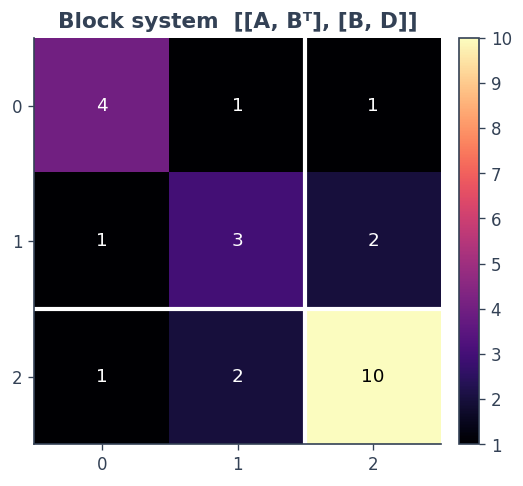
eigenvalues: [ 2.165 4.081 10.755] → SPD, so CG applies
3 · Solve it with conjugate gradients over the tree#
sc.cg does not care that the unknown is a tree — it only needs
M.apply and the tree inner product. The right-hand side and the
solution are tree elements.
b = (ctx.asarray([1.0, -2.0]), ctx.asarray([0.5]))     # RHS as a tree element
res = sc.cg(M, b, tol=1e-12, maxiter=50)

print("converged :", bool(res.converged), " iterations:", int(res.num_iters))
print("u block   :", res.x[0])
print("p block   :", res.x[1])

# cross-check against a plain dense solve on the flattened system
ref = np.linalg.solve(full, np.array([1.0, -2.0, 0.5]))
print("matches dense solve:", np.allclose(T.flatten(res.x), ref))
converged : True  iterations: 4
u block   : [ 0.43684211 -0.94210526]
p block   : [0.19473684]
matches dense solve: True
ks = np.arange(1, 7)
hist = [float(sc.cg(M, b, tol=0.0, atol=0.0, maxiter=int(k), check_every=1).residual_norm)
        for k in ks]

fig, axes = plt.subplots(1, 2, figsize=(10.2, 3.9))
axes[0].semilogy(ks, hist, color=BLUE, marker="o")
axes[0].set_title("CG residual over the tree space"); axes[0].set_xlabel("iteration")
axes[0].set_ylabel("residual (log)")

labels = ["u₁", "u₂", "p₁"]
axes[1].bar(labels, T.flatten(res.x), color=[BLUE, BLUE, PINK])
axes[1].axhline(0, color=SLATE, lw=1)
axes[1].set_title("Solution, split by leaf"); axes[1].set_ylabel("value")
plt.tight_layout(); plt.show()
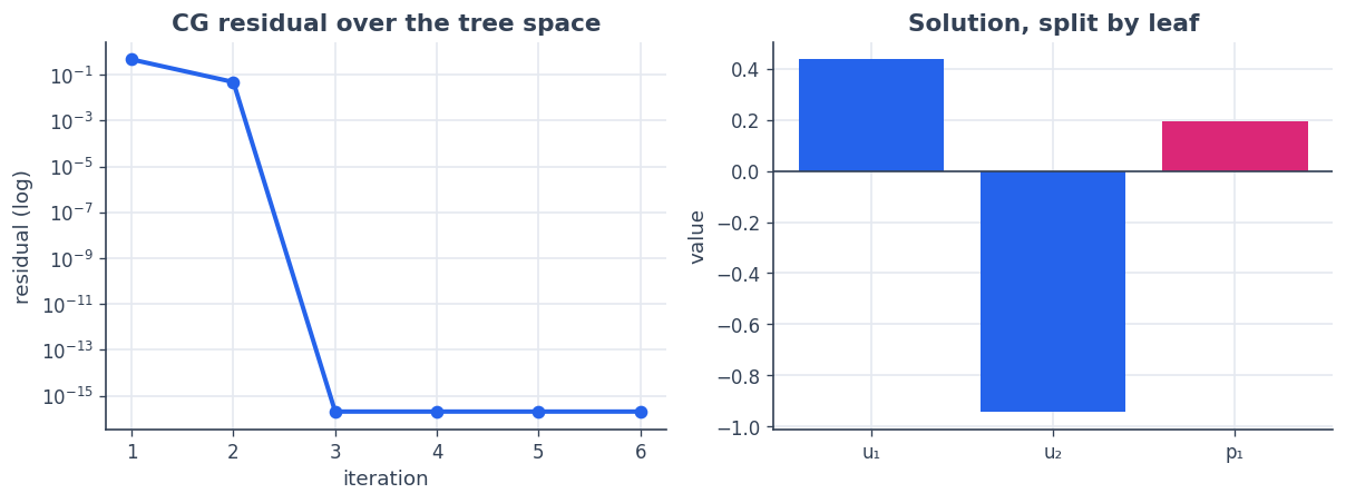
The two u bars (blue) and the p bar (pink) come back in their
own leaves — the solver never flattened your problem into an anonymous
vector.
4 · Named blocks#
A tuple tree is fine, but the blocks here mean something — a primal
state and a dual multiplier. A TreeSpace can carry that
naming: build it from a NamedTuple template with from_template,
and elements round-trip as that type, so you read blocks by name
instead of by position. The geometry, operators, and solvers are exactly
the same — only your access pattern changes.
from typing import NamedTuple

class KKT(NamedTuple):
    state: object        # the u block, in X = ℝ²
    multiplier: object   # the p block, in S = ℝ¹

T_named = sc.TreeSpace.from_template(KKT(0, 0), (X, S), ctx=ctx)

xb = T_named.element(KKT(state=ctx.asarray([1.0, 2.0]),
                         multiplier=ctx.asarray([3.0])))

print("element type :", type(xb.value).__name__)         # KKT — the original type
print("read by name :", xb.value.state, "|", xb.value.multiplier)
print("inner         :", T_named.inner(xb.value, xb.value))
print("same as tuple :", float(T_named.inner(xb.value, xb.value))
                          == float(T.inner((xb.value.state, xb.value.multiplier),
                                           (xb.value.state, xb.value.multiplier))))
element type : KKT
read by name : [1. 2.] | [3.]
inner         : 14.0
same as tuple : True
Dicts work as well —
sc.TreeSpace({"state": 0, "multiplier": 0}, (X, S), ctx=ctx) — with
one caveat: dict leaves are ordered by sorted key, so check
T.leaf_paths to confirm how leaf_spaces pairs up. A
NamedTuple keeps your declared field order, which is usually what
you want.
Recap#
A ``TreeSpace`` is a direct product of heterogeneous leaves; elements are Python trees and
inner/normsum over leaves.flatten/unflattenbridge to a plain vector.``BlockMatrixLinOp`` (and friends
BlockDiagonalLinOp,StackedLinOp,SumToSingleLinOp) compose leaf operators into maps between tree spaces.Solvers like ``sc.cg`` run unchanged over tree spaces — structure is preserved end to end.
Next: 5 · Weighted Tikhonov — a worked inverse problem where the metric adjoint does the heavy lifting.