6 · Optimal transport with a matrix-free operator#
Optimal transport asks how to move mass from a source distribution \(a\) to a target \(b\) at least cost. A transport plan is a nonnegative matrix \(P \in \mathbb{R}^{n\times m}\) whose row sums are \(a\) and column sums are \(b\):
Those two constraints are a single linear operator acting on the plan,
and it would be wasteful to store it as an \((n+m)\times nm\) matrix. This is the perfect job for a ``MatrixFreeLinOp``: we give SpaceCore the forward action and its adjoint as two small functions. We then solve entropic OT with the Sinkhorn algorithm, in which that operator’s adjoint is exactly the step that turns dual potentials into a transport plan.
You will learn to express marginalisation as a matrix-free operator, verify its adjoint, and use it inside a real algorithm.
import numpy as np
import matplotlib as mpl
import matplotlib.pyplot as plt
import spacecore as sc

# A clean, consistent palette + style for every figure in the tutorials.
BLUE, INDIGO, CYAN = "#2563eb", "#4f46e5", "#0891b2"
PINK, AMBER, GREEN = "#db2777", "#d97706", "#059669"
SLATE, GRID = "#334155", "#e5e9f0"

mpl.rcParams.update({
    "figure.figsize": (7.2, 4.2), "figure.dpi": 120, "savefig.dpi": 120,
    "figure.facecolor": "white", "axes.facecolor": "white",
    "axes.edgecolor": SLATE, "axes.linewidth": 1.0,
    "axes.grid": True, "axes.axisbelow": True,
    "grid.color": GRID, "grid.linewidth": 1.0,
    "axes.spines.top": False, "axes.spines.right": False,
    "axes.titlesize": 13, "axes.titleweight": "bold", "axes.titlecolor": SLATE,
    "axes.labelcolor": SLATE, "axes.labelsize": 11,
    "xtick.color": SLATE, "ytick.color": SLATE,
    "xtick.labelsize": 10, "ytick.labelsize": 10, "font.size": 11,
    "legend.frameon": False, "legend.fontsize": 10,
    "lines.linewidth": 2.4, "lines.markersize": 6, "image.cmap": "magma",
})
mpl.rcParams["axes.prop_cycle"] = mpl.cycler(
    color=[BLUE, PINK, GREEN, AMBER, INDIGO, CYAN])

print("spacecore", sc.__version__, "| numpy", np.__version__)
spacecore 0.4.0 | numpy 2.4.2
ctx = sc.Context(sc.NumpyOps(), dtype=np.float64)
ops = ctx.ops
1 · A source, a target, and a cost#
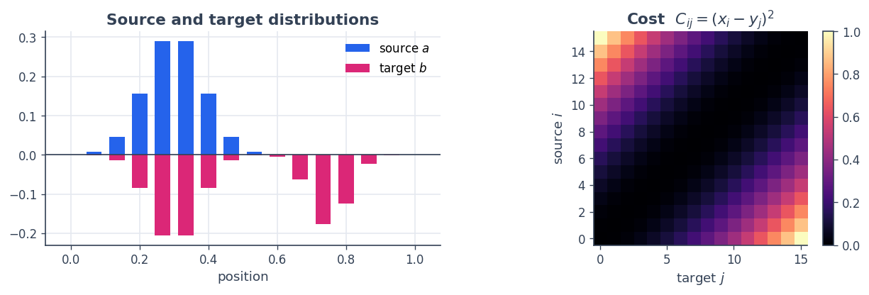
We place \(n\) source bins and \(m\) target bins on the line \([0,1]\). The source is a single bump, the target is bimodal. The cost to move a unit of mass from \(x_i\) to \(y_j\) is the squared distance \(C_{ij} = (x_i - y_j)^2\).
n, m = 16, 16
xs = np.linspace(0, 1, n)
ys = np.linspace(0, 1, m)

def normalize(v): return v / v.sum()
a = normalize(np.exp(-((xs - 0.30) / 0.12) ** 2))                       # source: one bump
b = normalize(np.exp(-((ys - 0.30) / 0.10) ** 2)
              + 0.8 * np.exp(-((ys - 0.75) / 0.08) ** 2))               # target: two bumps
Cmat = (xs[:, None] - ys[None, :]) ** 2                                 # cost matrix

fig, axes = plt.subplots(1, 2, figsize=(10.4, 3.6))
axes[0].bar(xs, a, width=0.045, color=BLUE, label="source $a$")
axes[0].bar(ys, -b, width=0.045, color=PINK, label="target $b$")
axes[0].axhline(0, color=SLATE, lw=1); axes[0].set_title("Source and target distributions")
axes[0].set_xlabel("position"); axes[0].legend()
im = axes[1].imshow(Cmat, cmap="magma", origin="lower"); axes[1].grid(False)
axes[1].set_title("Cost  $C_{ij}=(x_i-y_j)^2$"); axes[1].set_xlabel("target $j$"); axes[1].set_ylabel("source $i$")
fig.colorbar(im, ax=axes[1], fraction=0.046, pad=0.04); plt.tight_layout(); plt.show()
2 · Marginalisation as a MatrixFreeLinOp#
The plan lives in the matrix space \(\mathbb{R}^{n\times m}\); the marginals live in \(\mathbb{R}^{n+m}\). The forward map stacks the row sums and column sums. Its adjoint is the “broadcast” map that takes a vector \((\phi,\psi)\) and spreads it back over the matrix as \(\phi_i + \psi_j\) — the transpose of summation is tiling.
P_space = sc.DenseCoordinateSpace((n, m), ctx)      # transport plans
M_space = sc.DenseVectorSpace((n + m,), ctx)        # stacked marginals [row; col]

def marginals(P):                                   # forward:  P → (P1, Pᵀ1)
    return ops.concatenate([ops.sum(P, axis=1), ops.sum(P, axis=0)])

def broadcast(g):                                   # adjoint:  (φ, ψ) → φ_i + ψ_j
    return g[:n][:, None] + g[n:][None, :]

K = sc.MatrixFreeLinOp(marginals, broadcast, P_space, M_space, ctx)

# Verify the adjoint identity  <K P, g> = <P, K* g>  (no matrix ever formed)
rng = np.random.default_rng(0)
P_test = ctx.asarray(rng.standard_normal((n, m)))
g_test = ctx.asarray(rng.standard_normal(n + m))
lhs = float(M_space.inner(K.apply(P_test), g_test))
rhs = float(P_space.inner(P_test, K.rapply(g_test)))
print(f"<K P, g> = {lhs:.10f}")
print(f"<P, K*g> = {rhs:.10f}")
print("adjoint identity holds:", np.isclose(lhs, rhs))
<K P, g> = -1.8810878180
<P, K*g> = -1.8810878180
adjoint identity holds: True
3 · Sinkhorn, powered by the adjoint#
Entropic OT solves
\(\min_P \langle C, P\rangle + \varepsilon\sum_{ij} P_{ij}\log P_{ij}\)
subject to the marginals. Its optimal plan has the form
\(P_{ij} = \exp\big((\phi_i + \psi_j - C_{ij})/\varepsilon\big)\) —
and \(\phi_i+\psi_j\) is precisely K.rapply([φ, ψ]). Sinkhorn
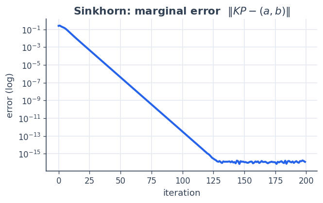
alternately rescales rows and columns to hit \(a\) and \(b\). We
track the marginal error with K.apply.
eps = 0.01
kernel = np.exp(-Cmat / eps)
u, v = np.ones(n), np.ones(m)
errors = []
for it in range(200):
    u = a / np.maximum(kernel @ v, 1e-300)
    v = b / np.maximum(kernel.T @ u, 1e-300)
    P = u[:, None] * kernel * v[None, :]
    err = float(M_space.norm(K.apply(ctx.asarray(P)) - ctx.asarray(np.concatenate([a, b]))))
    errors.append(err)

print("final marginal error :", errors[-1])
print("transport cost <C,P>  :", float(np.sum(Cmat * P)))

# the dual-potential form really does reproduce the plan, via the adjoint
phi, psi = eps * np.log(u), eps * np.log(v)
P_dual = np.exp((np.asarray(K.rapply(ctx.asarray(np.concatenate([phi, psi])))) - Cmat) / eps)
print("plan == exp((K* potentials − C)/ε):", np.allclose(P, P_dual))
final marginal error : 1.1943853798950167e-16
transport cost <C,P>  : 0.05880594096841237
plan == exp((K* potentials − C)/ε): True
fig, ax = plt.subplots(figsize=(6.0, 3.4))
ax.semilogy(errors, color=BLUE)
ax.set_title("Sinkhorn: marginal error  $\\|K P - (a,b)\\|$")
ax.set_xlabel("iteration"); ax.set_ylabel("error (log)"); plt.show()
4 · The transport plan#
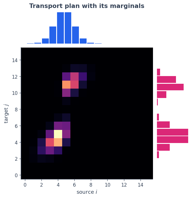
The coupling sits between the two marginals. We display it with the source on the horizontal axis and the target on the vertical axis, so the source marginal \(a\) sits on top and the target marginal \(b\) runs up the right — each aligned with the axis it belongs to. Mass flows from the single source bump to both target bumps.
from matplotlib.gridspec import GridSpec
fig = plt.figure(figsize=(6.4, 6.4))
gs = GridSpec(2, 2, width_ratios=[4, 1], height_ratios=[1, 4],
              wspace=0.05, hspace=0.05)
ax_top = fig.add_subplot(gs[0, 0]); ax_main = fig.add_subplot(gs[1, 0])
ax_right = fig.add_subplot(gs[1, 1])

# transpose the plan so the x-axis is the source and the y-axis is the target
ax_main.imshow(P.T, cmap="magma", origin="lower", aspect="auto"); ax_main.grid(False)
ax_main.set_xlabel("source $i$"); ax_main.set_ylabel("target $j$")
ax_top.bar(np.arange(n), a, color=BLUE, width=0.9); ax_top.axis("off")       # source marginal
ax_top.set_title("Transport plan with its marginals")
ax_right.barh(np.arange(m), b, color=PINK, height=0.9); ax_right.axis("off") # target marginal
plt.show()
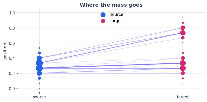
A second view makes the movement explicit: each ribbon connects a source bin to a target bin, with width proportional to the transported mass \(P_{ij}\).
fig, ax = plt.subplots(figsize=(8.4, 3.8))
Pn = P / P.max()
for i in range(n):
    for j in range(m):
        if Pn[i, j] > 0.02:
            ax.plot([0, 1], [xs[i], ys[j]], color=INDIGO,
                    alpha=float(min(Pn[i, j], 1.0)) * 0.7, lw=2.2 * Pn[i, j])
ax.scatter(np.zeros(n), xs, s=900 * a, color=BLUE, zorder=5, label="source")
ax.scatter(np.ones(m),  ys, s=900 * b, color=PINK, zorder=5, label="target")
ax.set_xlim(-0.15, 1.15); ax.set_xticks([0, 1]); ax.set_xticklabels(["source", "target"])
ax.set_ylabel("position"); ax.set_title("Where the mass goes"); ax.legend(loc="upper center")
plt.show()
Recap#
The OT marginal constraint is a linear operator \(K\);
MatrixFreeLinOp(apply, rapply, …)captures it with two tiny functions and no stored matrix.rapplymust be the true adjoint — here the broadcast/tiling map — and we checked the identity \(\langle KP, g\rangle = \langle P, K^\*g\rangle\) numerically.That same adjoint is the workhorse inside Sinkhorn: it assembles the plan \(P=\exp((K^\*[\phi,\psi]-C)/\varepsilon)\) from the dual potentials.
Next: 7 · Manifold descent — optimisation with a genuinely non-Euclidean geometry.